Below you can find the report and the code of my first attempt at a Kaggle competition. Feedback and recommendations are welcomed!
Competition selection
Link to the dataset: https://www.kaggle.com/c/forest-cover-type-prediction/data.
I selected this dataset because of the big number of variables to explore and use in my model, and because the data seemed very clean. I also liked the challenge of predicting a multi-categorical target feature. The competition has been around since 2015, meaning I was able to find a good amount of posts in the “Discussion” section of the competition, to learn and improve.
The description of the seven levels of the target feature are the following. In the dataset, however, are expressed in integers in the last column “Cover_Type”:
- Spruce/Fir
- Lodgepole Pine
- Ponderosa Pine
- Cottonwood/Willow
- Aspen
- Douglas-fir
- Krummholz
The “train” set of the competition includes 15,120 observations, while the “test” set 565,892 observations. The descriptive features are, in order:
- Elevation – Elevation in meters
- Aspect – Aspect in degrees azimuth
- Slope – Slope in degrees
- Horizontal_Distance_To_Hydrology – Horz Dist to nearest surface water features
- Vertical_Distance_To_Hydrology – Vert Dist to nearest surface water features
- Horizontal_Distance_To_Roadways – Horz Dist to nearest roadway
- Hillshade_9am (0 to 255 index) – Hillshade index at 9am, summer solstice
- Hillshade_Noon (0 to 255 index) – Hillshade index at noon, summer solstice
- Hillshade_3pm (0 to 255 index) – Hillshade index at 3pm, summer solstice
- Horizontal_Distance_To_Fire_Points – Horz Dist to nearest wildfire ignition points
- Wilderness_Area (4 binary columns, 0 = absence or 1 = presence) – Wilderness area designation
- Soil_Type (40 binary columns, 0 = absence or 1 = presence) – Soil Type designation
- Cover_Type (7 types, integers 1 to 7) – Forest Cover Type designation
Data exploration
One of the first element I checked through visualisation was the balance of the dataset. I discovered that the dataset was perfectly balanced: the 7 levels of the target feature had the same number of observations across the “train” dataset.


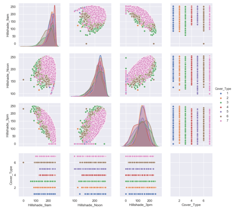
With the help of visualisation, I discovered interesting relationships between “Aspect”, “Hillshade” columns (3), and the columns describing horizontal distances.

As I did not encounter normal distributions, I decided to not investigate for outliers, as their presence could be beneficial to my model. The histograms visualised of continuous features, also, did not show to me concerning outliers.
The only two categorical features of the dataset, “Soil_Type” and “Wilderness_Area”, were already
one-hot encoded by the dataset provider in binary columns. Even if this type of encoding is ideal for the KNN algorithm, it aggravates the issue of dimensionality, especially for the “Soil_Type” category (consisting of 40 levels). For this reason, I decided to reverse this encoding by creating two new columns: “Soil_Type_All” and “Wilderness_Area_All”; I will test the two types of encodings in my iterations to assess what works best.
# I reverse the one-hot encoding of Soil_Type and Wilderness_Area, creating two new columns
soil_start = trees.columns.get_loc("Soil_Type1")
soil_end = trees.columns.get_loc("Soil_Type40")
trees.insert(soil_end+1,'Soil_Type_All', trees.iloc[:, soil_start:-1].idxmax(1))
area_start = trees.columns.get_loc("Wilderness_Area1")
area_end = trees.columns.get_loc("Wilderness_Area4")
trees.insert(area_end+1,'Wilderness_Area_All', trees.iloc[:, area_start:area_end+1].idxmax(1))
The model: K-nearest neighbour
Because of the high number of continuous features in the dataset, I decided to go with a similarity-based learning, in particular K-nearest neighbour.
As first step, I normalised the continuous features, as the KNN is very sensitive to not-normalised data.
I transformed the values in the newly created categorical columns in integers, in order to be utilised by my model. I was conscious this is not ideal, as it would imply an order between the levels of the categories; however, I still thought that it was better than train the model on too many features.
Before running the first iterations, for local evaluation purposes, I split the “train.csv” dataset in train (80%) and test (20%) data. In order to maintain the target feature balance, I used the parameter “stratify” of the “train_test_split” function.
Model iterations
Being a perfectly balanced dataset, I knew I could try high “k” values. My first iteration (“M1”) involved trying different values for “k”. I iterated through 3,5,6 and 8; and discovered that the best value of “k” was 5, as the model gave me an accuracy of 76%.
My second iteration involved trying a different distance metric than Euclidean: the Manhattan, as the latter is less influenced by single large differences in single features. The model accuracy was 74%, less than before. For this reason, I decided to use the Euclidean distance (default) for my following iterations.
For my third iteration, I decided to reduce the number of features on which to train the model, with the help of the SkLearn function “SelectKBest”. The function selected for me the top 8 features (out of 10), the accuracy of the third model (“M3”) was still just above 76%.
# I use the SelectKBest function to select the most 8 useful features for my model
selector = SelectKBest(chi2, k=8)
selector.fit(X_train, y_train)
cols = selector.get_support(indices=True)
X_train_new = X_train.iloc[:,cols]

sel_col = []
for col in X_train_new:
    sel_col.append(X_test.columns.get_loc(X_train_new[col].name))

# KNN classifier built with the previous selected features only
mod3 = KNeighborsClassifier(n_neighbors=5)
mod3.fit(X_train_new, y_train)
y_pred = mod3.predict(X_test.iloc[:,sel_col])
print("M3 Accuracy score: " + str(accuracy_score(y_test, y_pred)))
Before proceeding with the 4th iteration, I tested the difference between feeding the model with the one-hot encoded features “Wilderness_Area” (4 binary columns), or use the created column “Wilderness_Area_All”, with integer encoding. The accuracy of the two KNN classifiers were exactly the same.
For my following iteration, I included the “Wilderness_Area_All” and “Soil_Type_All” features in the model training. This greatly improved my model (“M4”), that scored an accuracy of 80%.
My 5th iteration involved changing the number of top features selected from 8 to 6. This proved to be successful, with an accuracy score for “M5” of 83%.
In my 6th iteration, I ran the same model but “distance-weighted” KNN algorithm, by adding the parameter “weights”. The reasoning was based on the fact the closer neighbours should have more weight in the distances calculation. “M6” was the most successful model found, scoring an accuracy of 85%.
# I test a distance weighted KNN
mod6 = KNeighborsClassifier(n_neighbors=5,weights='distance')
mod6.fit(X_train_new, y_train)
y_pred = mod6.predict(X_test.iloc[:,sel_col])
print("M6 Accuracy score: " + str(accuracy_score(y_test, y_pred)))
After checking single-class accuracy, I noticed that for three classes I achieved an accuracy of over 95%, while for one my accuracy was only 67%. This is an interesting point for future investigations.

The best performing KNN model found, at the end of all iterations, was “M6”.
Kaggle performance report
I ran my model on the Kaggle competition “test” dataset, and submitted my predictions. My score was 0.68217. This result was slightly disappointing, given the high accuracy achieved in my local evaluation of the model.

Future improvements
With more at my disposal, I would improve my model in the following ways:
- Use of 10-fold cross-validation in my local evaluation strategy.
- Deeper data exploration, by:
- better investigating features relationships and correlation.
- Investigate outliers, even if the distributions of continuous features are not-normal.
- Features engineering: I would create new features that would describe the relationship between the original features, and use them to train my model.
- Investigate low-accuracy classes predictions, by looking at the model accuracy by class.
- Testing a decision tree algorithm, after binning the continuous descriptive features.
- Group the 40 different “Soil_Types” in fewer categories.
Full code
import pandas as pd
import numpy as np
import matplotlib . pyplot as plt
import seaborn as sns
import math
from sklearn import preprocessing
from sklearn.model_selection import train_test_split
from sklearn.neighbors import KNeighborsClassifier
from sklearn.metrics import accuracy_score
from sklearn.datasets import load_iris
from sklearn.feature_selection import SelectKBest
from sklearn.feature_selection import chi2
from sklearn.metrics import confusion_matrix


# I import the training data, and check its main characteristics
trees = pd.read_csv("train.csv")
print(trees.shape)
trees = trees.set_index('Id')
print(trees.shape)
trees.dtypes
print(trees.describe())

# Check for missing values
trees.isnull().any()

# A funtion to check min and max of each feature
for column in trees:
    print(column + ': ' + str(trees[column].min()) + ' - ' + str(trees[column].max()))

# I reverse the one-hot encoding of Soil_Type and Wilderness_Area, creating two new columns
soil_start = trees.columns.get_loc("Soil_Type1")
soil_end = trees.columns.get_loc("Soil_Type40")
trees.insert(soil_end+1,'Soil_Type_All', trees.iloc[:, soil_start:-1].idxmax(1))
area_start = trees.columns.get_loc("Wilderness_Area1")
area_end = trees.columns.get_loc("Wilderness_Area4")
trees.insert(area_end+1,'Wilderness_Area_All', trees.iloc[:, area_start:area_end+1].idxmax(1))

# Visualise the target feature and the categorical feature Wilderness_Area
fig, ax = plt.subplots(1, 2, figsize=(17, 5))
ax[0].bar(trees['Cover_Type'].unique(), trees['Cover_Type'].value_counts())
ax[1].bar(trees['Wilderness_Area_All'].unique(), trees['Wilderness_Area_All'].value_counts())
plt.show()

# Visualise all continuous descriptive features
fig, ax = plt.subplots(2, 4,figsize=(17, 6))

ax[0,0].hist(trees.iloc[:,0])
ax[0,0].set_title(trees.columns[0])
ax[0,1].hist(trees.iloc[:,1])
ax[0,1].set_title(trees.columns[1])
ax[0,2].hist(trees.iloc[:,2])
ax[0,2].set_title(trees.columns[2])
ax[0,3].hist(trees.iloc[:,3])
ax[0,3].set_title(trees.columns[3])
ax[1,0].hist(trees.iloc[:,4])
ax[1,0].set_title(trees.columns[4])
ax[1,1].hist(trees.iloc[:,5])
ax[1,1].set_title(trees.columns[5])
ax[1,2].hist(trees.iloc[:,9])
ax[1,2].set_title(trees.columns[9])
ax[1,3].axis('off')

plt.tight_layout(h_pad=3)
plt.show()

# Visualise in detail Elevation and Aspect
fig, ax = plt.subplots(1, 2,figsize=(20, 8))

ax[0].hist(trees.iloc[:,0], bins=30)
ax[0].set_title(trees.columns[0])
ax[1].hist(trees.iloc[:,1], bins=30)
ax[1].set_title(trees.columns[1])

plt.show()

# Huge pairwise relationships plot of all continuous values; it may take time to load
sns.set()
#sns_plot = sns.pairplot(trees.iloc[:,0:10])
#sns_plot.savefig("pairplot.png")

# Detail of interesting relationships, with detail target feature plotted with color
sns.pairplot(trees.iloc[:,[0,1,56]], hue='Cover_Type');
sns.pairplot(trees.iloc[:,[6,7,8,56]], hue='Cover_Type');

# Histogram of main continuous features with the Cover_Type dimension on color
trees.pivot(columns="Cover_Type", values="Aspect").plot.hist(bins=50)
plt.show()
trees.pivot(columns="Cover_Type", values="Slope").plot.hist(bins=50)
plt.show()
trees.pivot(columns="Cover_Type", values="Elevation").plot.hist(bins=50)
plt.show()
trees.pivot(columns="Cover_Type", values="Hillshade_Noon").plot.hist(bins=50)
plt.show()
trees.pivot(columns="Cover_Type", values="Horizontal_Distance_To_Hydrology").plot.hist(bins=50)
plt.show()
trees.pivot(columns="Cover_Type", values="Vertical_Distance_To_Hydrology").plot.hist(bins=50)
plt.show()
trees.pivot(columns="Cover_Type", values="Horizontal_Distance_To_Roadways").plot.hist(bins=50)
plt.show()
trees.pivot(columns="Cover_Type", values="Horizontal_Distance_To_Fire_Points").plot.hist(bins=50)
plt.show()

# Boxplots of main continuous features by Cover_Type
plt.clf()
sns.boxplot(x="Cover_Type", y="Slope", data=trees)
plt.show()
plt.clf()
sns.boxplot(x="Cover_Type", y="Elevation", data=trees)
plt.show()
plt.clf()
sns.boxplot(x="Cover_Type", y="Aspect", data=trees)
plt.show()
plt.clf()
sns.boxplot(x="Cover_Type", y="Hillshade_Noon", data=trees)
plt.show()
plt.clf()
sns.boxplot(x="Cover_Type", y="Horizontal_Distance_To_Hydrology", data=trees)
plt.show()
plt.clf()

# Normalisation of continuous features
min_max_scaler = preprocessing.MinMaxScaler()
trees.iloc[:,:10] = min_max_scaler.fit_transform(trees.iloc[:,:10])

# I transform the categorical values in integers
trees['Wilderness_Area_All'] = trees['Wilderness_Area_All'].str.replace('Wilderness_Area','').astype(int)
trees['Soil_Type_All'] = trees['Soil_Type_All'].str.replace('Soil_Type','').astype(int)

# I select the first 10 features, and split the dataset in training and test, for local evaluation purposes
X_train, X_test, y_train, y_test = train_test_split(trees.iloc[:,:10], trees.iloc[:,-1], stratify=trees.iloc[:,-1], test_size=0.20, random_state=1)

# I test various k values
# First KNN classifier with K = 3, Euclidean distance (default)
mod1 = KNeighborsClassifier(n_neighbors=3)
mod1.fit(X_train, y_train)
y_pred = mod1.predict(X_test)
print("M1 K3 Accuracy score: " + str(accuracy_score(y_test, y_pred)))

# KNN classifier with K = 5
mod1 = KNeighborsClassifier(n_neighbors=5)
mod1.fit(X_train, y_train)
y_pred = mod1.predict(X_test)
print("M1 K5 Accuracy score: " + str(accuracy_score(y_test, y_pred)))

# First KNN classifier with K = 6
mod1 = KNeighborsClassifier(n_neighbors=6)
mod1.fit(X_train, y_train)
y_pred = mod1.predict(X_test)
print("M1 K6 Accuracy score: " + str(accuracy_score(y_test, y_pred)))

# First KNN classifier with K = 8
mod1 = KNeighborsClassifier(n_neighbors=8)
mod1.fit(X_train, y_train)
y_pred = mod1.predict(X_test)
print("M1 K8 Accuracy score: " + str(accuracy_score(y_test, y_pred)))

# I test a different type of distance metric
# KNN classifier with K = 5, manhattan distance
mod2 = KNeighborsClassifier(n_neighbors=5, metric="manhattan")
mod2.fit(X_train, y_train)
y_pred = mod2.predict(X_test)
print("M2 Accuracy score: " + str(accuracy_score(y_test, y_pred)))


# I use the SelectKBest function to select the most 8 useful features for my model
selector = SelectKBest(chi2, k=8)
selector.fit(X_train, y_train)
cols = selector.get_support(indices=True)
X_train_new = X_train.iloc[:,cols]

sel_col = []
for col in X_train_new:
    sel_col.append(X_test.columns.get_loc(X_train_new[col].name))

# KNN classifier built with the previous selected features only
mod3 = KNeighborsClassifier(n_neighbors=5)
mod3.fit(X_train_new, y_train)
y_pred = mod3.predict(X_test.iloc[:,sel_col])
print("M3 Accuracy score: " + str(accuracy_score(y_test, y_pred)))

# Test to assess the impact of two different encodings for the categorical values
# KNN with "Wilderness_Area" encoded in integers a single column
print(trees.columns.get_loc("Wilderness_Area_All"))
X_train, X_test, y_train, y_test = train_test_split(trees.iloc[:,[0,1,2,3,4,14]], trees.iloc[:,-1], stratify=trees.iloc[:,-1], test_size=0.20, random_state=1)
modt = KNeighborsClassifier(n_neighbors=5)
modt.fit(X_train, y_train)
y_pred = modt.predict(X_test)
print("Test with 'integer' encoding accuracy score: " + str(accuracy_score(y_test, y_pred)))

# KNN with "Wilderness_Area" one-hot encoded, as it was originally in the dataset
X_train, X_test, y_train, y_test = train_test_split(trees.iloc[:,[0,1,2,3,4,10,11,12,13]], trees.iloc[:,-1], stratify=trees.iloc[:,-1], test_size=0.20, random_state=1)
modt2 = KNeighborsClassifier(n_neighbors=5)
modt2.fit(X_train, y_train)
y_pred = modt2.predict(X_test)
print("Test with 'one-hot' encoding accuracy score: " + str(accuracy_score(y_test, y_pred)))


# For the next classifier, I include the "Wilderness_Area_All" and "Soil_Type_All" features
X_train, X_test, y_train, y_test = train_test_split(trees.iloc[:,[0,1,2,3,4,5,6,7,8,9,14,55]], trees.iloc[:,-1], stratify=trees.iloc[:,-1], test_size=0.20, random_state=1)
mod4 = KNeighborsClassifier(n_neighbors=5)
mod4.fit(X_train, y_train)
y_pred = mod4.predict(X_test)
print("M4 Accuracy score: " + str(accuracy_score(y_test, y_pred)))

# I repeat the process of automatic feature selection, but this time I select 6 instead of 8 top features
selector = SelectKBest(chi2, k=6)
selector.fit(X_train, y_train)
cols = selector.get_support(indices=True)
X_train_new = X_train.iloc[:,cols]

sel_col = []
for col in X_train_new:
    sel_col.append(X_test.columns.get_loc(X_train_new[col].name))

mod5 = KNeighborsClassifier(n_neighbors=5)
mod5.fit(X_train_new, y_train)
y_pred = mod5.predict(X_test.iloc[:,sel_col])
print("M5 Accuracy score: " + str(accuracy_score(y_test, y_pred)))

# I test a distance weighted KNN
mod6 = KNeighborsClassifier(n_neighbors=5,weights='distance')
mod6.fit(X_train_new, y_train)
y_pred = mod6.predict(X_test.iloc[:,sel_col])
print("M6 Accuracy score: " + str(accuracy_score(y_test, y_pred)))

# Check single class accuracy
m = confusion_matrix(y_test, y_pred)
cm = cm.astype('float') / cm.sum(axis=1)[:, np.newaxis]
print(cm.diagonal())

# I create a new "Hillshade" column, by averaging "Hillshade_9am", "Hillshade_Noon" and "Hillshade_3pm"
shade_start = trees.columns.get_loc("Hillshade_9am")
shade_end = trees.columns.get_loc("Hillshade_3pm")
trees.insert(shade_end+1,'Hillshade_Avg', (trees.iloc[:,shade_start] + trees.iloc[:,shade_start+1] + trees.iloc[:,shade_end])/3)

# KNN classifier that includes the newly created feature
X_train, X_test, y_train, y_test = train_test_split(trees.iloc[:,[0,1,2,3,4,5,9,10,15,56]], trees.iloc[:,-1], stratify=trees.iloc[:,-1], test_size=0.20, random_state=1)

selector2 = SelectKBest(chi2, k=6)
selector2.fit(X_train, y_train)
cols2 = selector2.get_support(indices=True)
X_train_new2 = X_train.iloc[:,cols2]

sel_col2 = []
for col in X_train_new2:
    sel_col2.append(X_test.columns.get_loc(X_train_new2[col].name))

mod7 = KNeighborsClassifier(n_neighbors=5,weights='distance')
mod7.fit(X_train_new2, y_train)
y_pred = mod7.predict(X_test.iloc[:,sel_col2])
print("M7 Accuracy score: " + str(accuracy_score(y_test, y_pred)))


# Preparation of the Kaggle test dataset, I make the same transformation made to the train dataset
kaggle_test = pd.read_csv("test.csv")
kaggle_test = kaggle_test.set_index('Id')
soil_start = kaggle_test.columns.get_loc("Soil_Type1")
soil_end = kaggle_test.columns.get_loc("Soil_Type40")
kaggle_test.insert(soil_end+1,'Soil_Type_All', kaggle_test.iloc[:, soil_start:-1].idxmax(1))
area_start = kaggle_test.columns.get_loc("Wilderness_Area1")
area_end = kaggle_test.columns.get_loc("Wilderness_Area4")
kaggle_test.insert(area_end+1,'Wilderness_Area_All', kaggle_test.iloc[:, area_start:area_end+1].idxmax(1))
kaggle_test.iloc[:,:10] = min_max_scaler.fit_transform(kaggle_test.iloc[:,:10])
kaggle_test['Wilderness_Area_All'] = kaggle_test['Wilderness_Area_All'].str.replace('Wilderness_Area','').astype(int)
kaggle_test['Soil_Type_All'] = kaggle_test['Soil_Type_All'].str.replace('Soil_Type','').astype(int)

# Dataset split and target feature prediction with the best model: "M6"
kaggle_test_sel = kaggle_test.iloc[:,[0,1,2,3,4,5,6,7,8,9,14,55]]

kaggle_pred = mod6.predict(kaggle_test_sel.iloc[:,sel_col])

# Export to CSV for submission
submission = {'Id': kaggle_test.index,
        'Cover_Type': kaggle_pred
        }

subm = pd.DataFrame(submission, columns = ['Id', 'Cover_Type'])

subm.to_csv(r'xxx.csv', index = True)